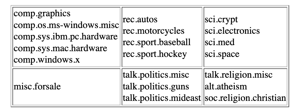
1) Merging labels according to the following table
!pip install spacy
!python -m spacy download en_core_web_md
!pip install wordcloud
Looking in indexes: https://pypi.org/simple, https://us-python.pkg.dev/colab-wheels/public/simple/
Requirement already satisfied: spacy in /usr/local/lib/python3.7/dist-packages (2.2.4)
Requirement already satisfied: cymem<2.1.0,>=2.0.2 in /usr/local/lib/python3.7/dist-packages (from spacy) (2.0.6)
Requirement already satisfied: srsly<1.1.0,>=1.0.2 in /usr/local/lib/python3.7/dist-packages (from spacy) (1.0.5)
Requirement already satisfied: catalogue<1.1.0,>=0.0.7 in /usr/local/lib/python3.7/dist-packages (from spacy) (1.0.0)
Requirement already satisfied: requests<3.0.0,>=2.13.0 in /usr/local/lib/python3.7/dist-packages (from spacy) (2.23.0)
Requirement already satisfied: preshed<3.1.0,>=3.0.2 in /usr/local/lib/python3.7/dist-packages (from spacy) (3.0.6)
Requirement already satisfied: thinc==7.4.0 in /usr/local/lib/python3.7/dist-packages (from spacy) (7.4.0)
Requirement already satisfied: murmurhash<1.1.0,>=0.28.0 in /usr/local/lib/python3.7/dist-packages (from spacy) (1.0.7)
Requirement already satisfied: numpy>=1.15.0 in /usr/local/lib/python3.7/dist-packages (from spacy) (1.21.6)
Requirement already satisfied: blis<0.5.0,>=0.4.0 in /usr/local/lib/python3.7/dist-packages (from spacy) (0.4.1)
Requirement already satisfied: plac<1.2.0,>=0.9.6 in /usr/local/lib/python3.7/dist-packages (from spacy) (1.1.3)
Requirement already satisfied: setuptools in /usr/local/lib/python3.7/dist-packages (from spacy) (57.4.0)
Requirement already satisfied: tqdm<5.0.0,>=4.38.0 in /usr/local/lib/python3.7/dist-packages (from spacy) (4.64.0)
Requirement already satisfied: wasabi<1.1.0,>=0.4.0 in /usr/local/lib/python3.7/dist-packages (from spacy) (0.9.1)
Requirement already satisfied: importlib-metadata>=0.20 in /usr/local/lib/python3.7/dist-packages (from catalogue<1.1.0,>=0.0.7->spacy) (4.11.3)
Requirement already satisfied: zipp>=0.5 in /usr/local/lib/python3.7/dist-packages (from importlib-metadata>=0.20->catalogue<1.1.0,>=0.0.7->spacy) (3.8.0)
Requirement already satisfied: typing-extensions>=3.6.4 in /usr/local/lib/python3.7/dist-packages (from importlib-metadata>=0.20->catalogue<1.1.0,>=0.0.7->spacy) (4.2.0)
Requirement already satisfied: urllib3!=1.25.0,!=1.25.1,<1.26,>=1.21.1 in /usr/local/lib/python3.7/dist-packages (from requests<3.0.0,>=2.13.0->spacy) (1.24.3)
Requirement already satisfied: chardet<4,>=3.0.2 in /usr/local/lib/python3.7/dist-packages (from requests<3.0.0,>=2.13.0->spacy) (3.0.4)
Requirement already satisfied: certifi>=2017.4.17 in /usr/local/lib/python3.7/dist-packages (from requests<3.0.0,>=2.13.0->spacy) (2022.5.18.1)
Requirement already satisfied: idna<3,>=2.5 in /usr/local/lib/python3.7/dist-packages (from requests<3.0.0,>=2.13.0->spacy) (2.10)
Looking in indexes: https://pypi.org/simple, https://us-python.pkg.dev/colab-wheels/public/simple/
Collecting en_core_web_md==2.2.5
  Downloading https://github.com/explosion/spacy-models/releases/download/en_core_web_md-2.2.5/en_core_web_md-2.2.5.tar.gz (96.4 MB)
     |████████████████████████████████| 96.4 MB 15.1 MB/s
Requirement already satisfied: spacy>=2.2.2 in /usr/local/lib/python3.7/dist-packages (from en_core_web_md==2.2.5) (2.2.4)
Requirement already satisfied: thinc==7.4.0 in /usr/local/lib/python3.7/dist-packages (from spacy>=2.2.2->en_core_web_md==2.2.5) (7.4.0)
Requirement already satisfied: numpy>=1.15.0 in /usr/local/lib/python3.7/dist-packages (from spacy>=2.2.2->en_core_web_md==2.2.5) (1.21.6)
Requirement already satisfied: catalogue<1.1.0,>=0.0.7 in /usr/local/lib/python3.7/dist-packages (from spacy>=2.2.2->en_core_web_md==2.2.5) (1.0.0)
Requirement already satisfied: tqdm<5.0.0,>=4.38.0 in /usr/local/lib/python3.7/dist-packages (from spacy>=2.2.2->en_core_web_md==2.2.5) (4.64.0)
Requirement already satisfied: wasabi<1.1.0,>=0.4.0 in /usr/local/lib/python3.7/dist-packages (from spacy>=2.2.2->en_core_web_md==2.2.5) (0.9.1)
Requirement already satisfied: setuptools in /usr/local/lib/python3.7/dist-packages (from spacy>=2.2.2->en_core_web_md==2.2.5) (57.4.0)
Requirement already satisfied: murmurhash<1.1.0,>=0.28.0 in /usr/local/lib/python3.7/dist-packages (from spacy>=2.2.2->en_core_web_md==2.2.5) (1.0.7)
Requirement already satisfied: blis<0.5.0,>=0.4.0 in /usr/local/lib/python3.7/dist-packages (from spacy>=2.2.2->en_core_web_md==2.2.5) (0.4.1)
Requirement already satisfied: requests<3.0.0,>=2.13.0 in /usr/local/lib/python3.7/dist-packages (from spacy>=2.2.2->en_core_web_md==2.2.5) (2.23.0)
Requirement already satisfied: plac<1.2.0,>=0.9.6 in /usr/local/lib/python3.7/dist-packages (from spacy>=2.2.2->en_core_web_md==2.2.5) (1.1.3)
Requirement already satisfied: srsly<1.1.0,>=1.0.2 in /usr/local/lib/python3.7/dist-packages (from spacy>=2.2.2->en_core_web_md==2.2.5) (1.0.5)
Requirement already satisfied: preshed<3.1.0,>=3.0.2 in /usr/local/lib/python3.7/dist-packages (from spacy>=2.2.2->en_core_web_md==2.2.5) (3.0.6)
Requirement already satisfied: cymem<2.1.0,>=2.0.2 in /usr/local/lib/python3.7/dist-packages (from spacy>=2.2.2->en_core_web_md==2.2.5) (2.0.6)
Requirement already satisfied: importlib-metadata>=0.20 in /usr/local/lib/python3.7/dist-packages (from catalogue<1.1.0,>=0.0.7->spacy>=2.2.2->en_core_web_md==2.2.5) (4.11.3)
Requirement already satisfied: typing-extensions>=3.6.4 in /usr/local/lib/python3.7/dist-packages (from importlib-metadata>=0.20->catalogue<1.1.0,>=0.0.7->spacy>=2.2.2->en_core_web_md==2.2.5) (4.2.0)
Requirement already satisfied: zipp>=0.5 in /usr/local/lib/python3.7/dist-packages (from importlib-metadata>=0.20->catalogue<1.1.0,>=0.0.7->spacy>=2.2.2->en_core_web_md==2.2.5) (3.8.0)
Requirement already satisfied: urllib3!=1.25.0,!=1.25.1,<1.26,>=1.21.1 in /usr/local/lib/python3.7/dist-packages (from requests<3.0.0,>=2.13.0->spacy>=2.2.2->en_core_web_md==2.2.5) (1.24.3)
Requirement already satisfied: chardet<4,>=3.0.2 in /usr/local/lib/python3.7/dist-packages (from requests<3.0.0,>=2.13.0->spacy>=2.2.2->en_core_web_md==2.2.5) (3.0.4)
Requirement already satisfied: certifi>=2017.4.17 in /usr/local/lib/python3.7/dist-packages (from requests<3.0.0,>=2.13.0->spacy>=2.2.2->en_core_web_md==2.2.5) (2022.5.18.1)
Requirement already satisfied: idna<3,>=2.5 in /usr/local/lib/python3.7/dist-packages (from requests<3.0.0,>=2.13.0->spacy>=2.2.2->en_core_web_md==2.2.5) (2.10)
Building wheels for collected packages: en-core-web-md
  Building wheel for en-core-web-md (setup.py) ... done
  Created wheel for en-core-web-md: filename=en_core_web_md-2.2.5-py3-none-any.whl size=98051301 sha256=653671f5fe614e69a3906328e1dd0a553bf1ae6f572513cdbdfc441479ba1136
  Stored in directory: /tmp/pip-ephem-wheel-cache-j16uorwl/wheels/69/c5/b8/4f1c029d89238734311b3269762ab2ee325a42da2ce8edb997
Successfully built en-core-web-md
Installing collected packages: en-core-web-md
Successfully installed en-core-web-md-2.2.5
✔ Download and installation successful
You can now load the model via spacy.load('en_core_web_md')
Looking in indexes: https://pypi.org/simple, https://us-python.pkg.dev/colab-wheels/public/simple/
Requirement already satisfied: wordcloud in /usr/local/lib/python3.7/dist-packages (1.5.0)
Requirement already satisfied: numpy>=1.6.1 in /usr/local/lib/python3.7/dist-packages (from wordcloud) (1.21.6)
Requirement already satisfied: pillow in /usr/local/lib/python3.7/dist-packages (from wordcloud) (7.1.2)
import pandas as pd
import numpy as np
from sklearn.preprocessing import LabelEncoder
from collections import Counter
import matplotlib.pyplot as plt
import spacy
from sklearn.model_selection import train_test_split
import gensim
from wordcloud import WordCloud, STOPWORDS
import matplotlib.colors as mcolors
from gensim.models.coherencemodel import CoherenceModel
from sklearn.linear_model import SGDClassifier
from sklearn.pipeline import Pipeline
from sklearn.feature_extraction.text import CountVectorizer
from sklearn.feature_extraction.text import TfidfTransformer
from sklearn.model_selection import GridSearchCV
from sklearn.metrics import confusion_matrix, f1_score, roc_curve, roc_auc_score, classification_report
import seaborn as sns
import warnings
warnings.filterwarnings("ignore")
Clasifying documents using topic models
In this notebook, the 20Newsgroup datasets will be used. It contains 20,000 documents with messages sent to different distribution lists. The dataset is available through Sklearn:
from sklearn.datasets import fetch_20newsgroups
newsgroups = fetch_20newsgroups(subset='all', shuffle = True, remove=('headers', 'footers', 'quotes'))
The documents could be accessed as follows:
print(type(newsgroups.data))

print('There are %d documents' %(len(newsgroups.data)))
<class 'list'>
There are 18846 documents
print(newsgroups.data[50])
WHen trying to choose a resistor with a tolerance better than 1%, you
need a trimmer or to screen devices, it can't be made from adding 2
resitors of 1% value in parallel, since the smaller device will have the
error of 1% to cope with.
You have 3 choices;
a) live with the error of 1% tolerance devices for low Q circuits or low
sensitivity designs
b) buy resistors with better than 1% tolerance (Vishay/Dale)
c) use trimmers or SOT's (Select-On-Test)
The documents are classified in 20 groups:
newsgroups.target
array([10, 3, 17, ..., 3, 1, 7])
df = pd.DataFrame({'Category':newsgroups.target_names,'Label':range(len(newsgroups.target_names))})
df
| Category | Label | |
|---|---|---|
| 0 | alt.atheism | 0 |
| 1 | comp.graphics | 1 |
| 2 | comp.os.ms-windows.misc | 2 |
| 3 | comp.sys.ibm.pc.hardware | 3 |
| 4 | comp.sys.mac.hardware | 4 |
| 5 | comp.windows.x | 5 |
| 6 | misc.forsale | 6 |
| 7 | rec.autos | 7 |
| 8 | rec.motorcycles | 8 |
| 9 | rec.sport.baseball | 9 |
| 10 | rec.sport.hockey | 10 |
| 11 | sci.crypt | 11 |
| 12 | sci.electronics | 12 |
| 13 | sci.med | 13 |
| 14 | sci.space | 14 |
| 15 | soc.religion.christian | 15 |
| 16 | talk.politics.guns | 16 |
| 17 | talk.politics.mideast | 17 |
| 18 | talk.politics.misc | 18 |
| 19 | talk.religion.misc | 19 |
In this notebook I will analyze the corpus from a topic modelling point of view and classify the documents:
1) Merging labels according to the similar groups.
2) Spliting the data in train (70%), validation (10%) and test (20%). Defining the dictionary using gensim and filter too-frequent tokens. Constructing the BoW representation of the model.
4) Building an LDA model for on the training set. Validating the number of topics, studying the consistency of the topics in the validation set. For the selected number of topics, studying their interpretability by analyzing the most likely words per topic.
5) Training a logistic regression and KNN classifier to classify each document using its LDA representation. Representing the confusion matrix in test and determining which categories are more problematic.
7) Comparing the results with a classifier that uses the TF-IDF representation.
In this part, the labels will be replaced to merge with new label values.
labels = newsgroups.target
mapping = {
  1: 100, 2: 100, 3: 100, 4: 100, 5: 100, #comp
  7: 200, 8: 200, 9: 200, 10: 200, #rec
  11: 300, 12: 300, 13:300, 14:300, # sci
  6: 400, # misc
  16: 500, 17: 500, 18: 500, # talk.politics
  19: 600, 0: 600, 15: 600 # religion
}
labels = [mapping.get(number, number) for number in labels]
np.unique(labels)
array([100, 200, 300, 400, 500, 600])
On the below dataframe, the new target names and labels could be seen:
new_target_names = ['computer_news','rec_news', 'science_news','misc_news','politics_news','religion_news']
new_labels = pd.DataFrame({'Category':new_target_names,'Label':np.unique(labels)})
new_labels
| Category | Label | |
|---|---|---|
| 0 | computer_news | 100 |
| 1 | rec_news | 200 |
| 2 | science_news | 300 |
| 3 | misc_news | 400 |
| 4 | politics_news | 500 |
| 5 | religion_news | 600 |
To check if everything is right, it could be seen that after replacing the labels, the number of documents is the same (18846)
len(labels)
18846
After replacing with specific values, using LabelEncoder, to make the labels again from 0 to 5.
le = LabelEncoder()
labels = le.fit_transform(labels)
new_labels["Label"] = np.unique(labels)
print(np.unique(labels))
new_labels
[0 1 2 3 4 5]
| Category | Label | |
|---|---|---|
| 0 | computer_news | 0 |
| 1 | rec_news | 1 |
| 2 | science_news | 2 |
| 3 | misc_news | 3 |
| 4 | politics_news | 4 |
| 5 | religion_news | 5 |
all_data = pd.DataFrame({'Texts':newsgroups.data,'Label':labels})
all_data_label_names = pd.merge(all_data, new_labels, on="Label",how="left")
all_data_label_names
| Texts | Label | Category | |
|---|---|---|---|
| 0 | \n\nI am sure some bashers of Pens fans are pr... | 1 | rec_news |
| 1 | My brother is in the market for a high-perform... | 0 | computer_news |
| 2 | \n\n\n\n\tFinally you said what you dream abou... | 4 | politics_news |
| 3 | \nThink!\n\nIt's the SCSI card doing the DMA t... | 0 | computer_news |
| 4 | 1) I have an old Jasmine drive which I cann... | 0 | computer_news |
| ... | ... | ... | ... |
| 18841 | DN> From: [email protected] (David Nye)\nD... | 2 | science_news |
| 18842 | \nNot in isolated ground recepticles (usually ... | 2 | science_news |
| 18843 | I just installed a DX2-66 CPU in a clone mothe... | 0 | computer_news |
| 18844 | \nWouldn't this require a hyper-sphere. In 3-... | 0 | computer_news |
| 18845 | After a tip from Gary Crum ([email protected].... | 1 | rec_news |
18846 rows × 3 columns
all_data_label_names.groupby(['Category',"Label"]).count()
| Texts | ||
|---|---|---|
| Category | Label | |
| computer_news | 0 | 4891 |
| misc_news | 3 | 975 |
| politics_news | 4 | 2625 |
| rec_news | 1 | 3979 |
| religion_news | 5 | 2424 |
| science_news | 2 | 3952 |
all_data_label_names.groupby(['Category',"Label"]).count().plot(kind='pie',shadow = True,subplots=True,
                                                      startangle=90,
                                                      figsize=(10,8), autopct='%1.1f%%')
array([<matplotlib.axes._subplots.AxesSubplot object at 0x7f7d2642ac10>],
      dtype=object)

As seen on the above pie chart, the classes are imbalanced. The least class is misc news (5.2%), on the other hand, computers (26%), rec news (21.1%) and science news(21%) are more than others. Moreover, politics and religion news ratio are more or less similar with 13.9% and 12.9%, respectively. Therefore, the least class is misc news and the highest frequent class is computer news.
Before splitting the data into train, validation and test, text preprocessing will be done. First, to speed up the preprocessing steps, the first characters per text will be kept. To define the limit character to keep, the average character in all the texts will be checked, and also the texts that have more than 5000 characters will be counted. Because it would be advisable keeping 5000 characters per text which is enough.
texts = newsgroups.data
length_texts = []
for i in range(len(texts)):
  length_texts = np.append(length_texts, len(texts[i]))
print('The average characters in the texts: ',length_texts.mean())
print('Maximum character in the texts:', max(length_texts))
count = sum(map(lambda x : x > 5000, length_texts))
print('Count of characters in the texts which are more than 5000:', count)
The average characters in the texts:  1169.667515653189
Maximum character in the texts: 158791.0
Count of characters in the texts which are more than 5000: 546
On the above results, it can be seen that the average character is around 1170, and the longest text has 158791 characters. The number of texts that have more than 5000 characters are 546. As there are 18846 texts, it is not that much. Therefore, these longer texts could decrease the speed of processing. It is better to limit the number of characters.
nlp = spacy.load('en_core_web_md')

list_processes = ["ner"]  # To speed up

for l in list_processes:
    nlp.disable_pipes(l)

limit = 5000
news_proc = [nlp(c[:limit]) if len(c)>limit else nlp(c) for c in texts]
In this part, for pre-processing, the spacy package will be used. As the texts are in English, en_core_web_md will be uploaded. Respectively, first the stopping words, punctuation marks and tokens with non-alphabetic characters will be removed.
def normalize(doc):
    return [w for w in doc if not w.is_stop and not w.is_punct and w.is_alpha] # Alphabetic tokens only

# we eliminate stop words, punctuations and tokens
news_norm = [normalize(c) for c in news_proc]

# We switch to text mode
news_text = [[w.lemma_.lower() for w in c] for c in news_norm]
print("Before Preprocessing:")
print(newsgroups.data[1])
print("------")
print("After Preprocessing:")
print(news_text[1])
Before Preprocessing:
My brother is in the market for a high-performance video card that supports
VESA local bus with 1-2MB RAM.  Does anyone have suggestions/ideas on:

  - Diamond Stealth Pro Local Bus

  - Orchid Farenheit 1280

  - ATI Graphics Ultra Pro

  - Any other high-performance VLB card


Please post or email.  Thank you!

  - Matt

------
After Preprocessing:
['brother', 'market', 'high', 'performance', 'video', 'card', 'support', 'vesa', 'local', 'bus', 'mb', 'ram', 'suggestion', 'idea', 'diamond', 'stealth', 'pro', 'local', 'bus', 'orchid', 'farenheit', 'ati', 'graphics', 'ultra', 'pro', 'high', 'performance', 'vlb', 'card', 'post', 'email', 'thank', 'matt']
Here, while splitting the data, first the data will be split into train and test with the ratio 80-20. Then to validate the number of topics in the following part, the training sample will be split into training and validation with the ratio 70-10. However, in the end, the model will be trained with 80% of the data and test the model with 20% of the data.
## First splitting into train and test
X_train, X_test, Y_train, Y_test = train_test_split(news_text, labels,
    test_size=0.2, shuffle = True, random_state = 100459259)

## Second splitting the train into train and validation sets
X_train_val, X_val, Y_train_val, Y_val = train_test_split(X_train, Y_train,
    test_size=0.125, random_state= 100459259) # 0.125 x 0.8 = 0.1

print("X_train shape: {}".format(len(X_train)))
print("Y_train shape: {}".format(len(Y_train)))
print("X_test shape: {}".format(len(X_test)))
print("Y_test shape: {}".format(len(Y_test)))
print("X_train_val shape: {}".format(len(X_train_val)))
print("Y_train_val shape: {}".format(len(Y_train_val)))
print("X_val shape: {}".format(len(X_val)))
print("Y_val shape: {}".format(len(Y_val)))
X_train shape: 15076
Y_train shape: 15076
X_test shape: 3770
Y_test shape: 3770
X_train_val shape: 13191
Y_train_val shape: 13191
X_val shape: 1885
Y_val shape: 1885
The dictionary on the training set.
D = gensim.corpora.Dictionary(X_train)

no_below = 5 # Minimum number of documents to keep a term in the dictionary
no_above = .75 # Maximum proportion of documents in which a term can appear to be kept in the dictionary
D.filter_extremes(no_below=no_below,no_above=no_above,keep_n=2000)

n_tokens = len(D)

print('The dictionary contains', n_tokens, 'terms')
print('First terms in the dictionary:')
for n in range(10):
    print(str(n), ':', D[n])
The dictionary contains 2000 terms
First terms in the dictionary:
0 : actually
1 : bad
2 : beat
3 : bit
4 : couple
5 : end
6 : fan
7 : final
8 : fun
9 : game
On the above, the 10 too-frequent tokens could be seen.
On the below, before building an LDA model on the training set, the corpus_bow for the training set will be created:
# the BoW representation of the corpus
corpus_bow = [D.doc2bow(doc) for doc in X_train]
#Plot BoW
print('Word counts for the document (first 10 components):')
list_word_counts = [(D[doc_bow[0]], doc_bow[1]) for doc_bow in corpus_bow[100][:10]] #100 documents
(words, counts) = zip(*list_word_counts)
plt.figure(figsize=(10,5))
plt.stem(words,counts, use_line_collection = True)
plt.xlabel('Words')
plt.ylabel('Counts')
plt.show()
Word counts for the document (first 10 components):

LDA is an unsupervised technique. LDA’s approach to topic modeling is that it considers each document as a collection of topics in a certain proportion. And each topic as a collection of keywords. Once in the algorithm, the number of topics is provided, all it does to rearrange the topics distribution within the documents and keywords distribution within the topics to obtain a good composition of topic-keywords distribution.
While I get the LDA base model, there are some parameters to be defined. As I have defined before the corpus and dictionary(id2word), I need to provide the number of topics (num_topics) as well. I set to 6 topics, however, I am going to evaluate the optimal number of topics in the following parts. chunksize controls how many documents are processed at a time in the training algorithm. Increasing chunksize will speed up training.
passes controls how often I train the model on the entire corpus. It defines the number of epochs. I set to 10.
lda_model = gensim.models.LdaMulticore(corpus_bow, num_topics=6, id2word = D, chunksize=300,passes=10)
for idx, topic in lda_model.print_topics(num_words=20):
    print("Topic: %d \nWords: %s" %(idx, topic))
    print("\n")
Topic: 0
Words: 0.034*"game" + 0.024*"team" + 0.023*"year" + 0.021*"play" + 0.016*"player" + 0.014*"win" + 0.012*"good" + 0.009*"hockey" + 0.009*"think" + 0.009*"fan" + 0.008*"season" + 0.008*"get" + 0.007*"hit" + 0.007*"time" + 0.007*"run" + 0.007*"lose" + 0.007*"goal" + 0.006*"division" + 0.006*"period" + 0.006*"score"


Topic: 1
Words: 0.016*"god" + 0.014*"people" + 0.012*"think" + 0.011*"know" + 0.010*"believe" + 0.009*"say" + 0.007*"mean" + 0.006*"man" + 0.006*"come" + 0.006*"way" + 0.006*"thing" + 0.006*"point" + 0.006*"life" + 0.006*"jesus" + 0.005*"question" + 0.005*"time" + 0.005*"like" + 0.005*"read" + 0.005*"right" + 0.005*"fact"


Topic: 2
Words: 0.014*"like" + 0.013*"think" + 0.011*"know" + 0.010*"good" + 0.010*"time" + 0.009*"go" + 0.008*"thing" + 0.008*"get" + 0.008*"car" + 0.007*"want" + 0.007*"year" + 0.006*"look" + 0.006*"problem" + 0.006*"way" + 0.005*"work" + 0.005*"people" + 0.005*"need" + 0.005*"high" + 0.005*"use" + 0.005*"come"


Topic: 3
Words: 0.017*"people" + 0.014*"gun" + 0.013*"government" + 0.013*"kill" + 0.011*"state" + 0.009*"say" + 0.009*"turkish" + 0.009*"right" + 0.009*"child" + 0.009*"fire" + 0.008*"war" + 0.008*"country" + 0.007*"law" + 0.007*"fbi" + 0.007*"armenian" + 0.007*"font" + 0.007*"soldier" + 0.006*"armenians" + 0.006*"crime" + 0.006*"house"


Topic: 4
Words: 0.013*"x" + 0.012*"drive" + 0.012*"file" + 0.012*"run" + 0.011*"use" + 0.010*"window" + 0.010*"problem" + 0.010*"work" + 0.009*"know" + 0.008*"system" + 0.008*"program" + 0.008*"card" + 0.008*"like" + 0.008*"thank" + 0.008*"try" + 0.007*"disk" + 0.007*"need" + 0.007*"windows" + 0.006*"dos" + 0.006*"help"


Topic: 5
Words: 0.017*"key" + 0.011*"information" + 0.010*"list" + 0.009*"space" + 0.009*"send" + 0.009*"chip" + 0.008*"program" + 0.008*"post" + 0.008*"mail" + 0.007*"system" + 0.007*"use" + 0.007*"public" + 0.007*"include" + 0.006*"article" + 0.006*"number" + 0.006*"available" + 0.006*"message" + 0.006*"technology" + 0.006*"phone" + 0.006*"university"
cols = [color for name, color in mcolors.TABLEAU_COLORS.items()]  # more colors: 'mcolors.XKCD_COLORS'

cloud = WordCloud(background_color='white',
                  width=2500,
                  height=1800,
                  max_words=20,
                  colormap='tab10',
                  color_func=lambda *args, **kwargs: cols[i],
                  prefer_horizontal=1.0)

topics = lda_model.show_topics(formatted=False,num_words=20)

fig, axes = plt.subplots(1, 6, figsize=(20,10), sharex=True, sharey=True)

for i, ax in enumerate(axes.flatten()):
    fig.add_subplot(ax)
    topic_words = dict(topics[i][1])
    cloud.generate_from_frequencies(topic_words, max_font_size=300)
    plt.gca().imshow(cloud)
    plt.gca().set_title('Topic ' + str(i), fontdict=dict(size=16))
    plt.gca().axis('off')


plt.subplots_adjust(wspace=0, hspace=0)
plt.axis('off')
plt.margins(x=0, y=0)
plt.tight_layout()
plt.show()

First, I need to define the corpus of train and validation sets. Then i am going to use these corpuses
corpus_bow_train = [D.doc2bow(doc) for doc in X_train_val] # %70
corpus_bow_val = [D.doc2bow(doc) for doc in X_val] # %10
corpus_bow_test = [D.doc2bow(doc) for doc in X_test] # %20
from gensim.models.coherencemodel import CoherenceModel

K_max = 11 ## maximum topics

L_CV = []

L_UCI = []

L_mass = []

L_NPMI = []

L_perp = []

L_CV_train = []

L_UCI_train = []

L_mass_train = []

L_NPMI_train = []

L_perp_train = []

topic_models = {}

for k in range(4,K_max,1):

    print(k)
    ## building an LDA model on the training set
    topic_models[k] = gensim.models.LdaMulticore(corpus_bow_train, num_topics=k, id2word = D, chunksize=300, passes=30, workers=7)

    #### Coherence score
    cv = CoherenceModel(model=topic_models[k], texts=X_val, dictionary=D, coherence='c_v')

    L_CV.append(cv.get_coherence())

    cv = CoherenceModel(model=topic_models[k], texts=X_train_val, dictionary=D, coherence='c_v')

    L_CV_train.append(cv.get_coherence())

    #### Perplexity

    L_perp.append(topic_models[k].log_perplexity(corpus_bow_val))

    L_perp_train.append(topic_models[k].log_perplexity(corpus_bow_train))

    #### UCI

    cm = CoherenceModel(model=topic_models[k], texts=X_val, dictionary=D, coherence='c_uci')

    L_UCI.append(cm.get_coherence())

    cm = CoherenceModel(model=topic_models[k], texts=X_train_val, dictionary=D, coherence='c_uci')

    L_UCI_train.append(cm.get_coherence())

    #### UMASS

    cm = CoherenceModel(model=topic_models[k], texts=X_val, dictionary=D, coherence='u_mass')

    L_mass.append(cm.get_coherence())

    cm = CoherenceModel(model=topic_models[k], texts=X_train_val, dictionary=D, coherence='u_mass')

    L_mass_train.append(cm.get_coherence())

    #### CNPMI

    cm = CoherenceModel(model=topic_models[k], texts=X_val, dictionary=D, coherence='c_npmi')

    L_NPMI.append(cm.get_coherence())

    cm = CoherenceModel(model=topic_models[k], texts=X_train_val, dictionary=D, coherence='c_npmi')

    L_NPMI_train.append(cm.get_coherence())
4
5
6
7
8
9
10
fig, axes = plt.subplots(2, 2, figsize=(12,16))
cols = [color for name, color in mcolors.TABLEAU_COLORS.items()]

axes[0,0].plot(range(4,K_max,1),L_perp,color=cols[0],label='Validation')
axes[0,0].plot(range(4,K_max,1),L_perp_train,'--',color=cols[0],label='Training')
axes[0,0].set_ylabel('log-perplexity')
axes[0,0].set_xlabel('Number of topics')
axes[0,0].legend()
axes[0,0].grid()

axes[0,1].plot(range(4,K_max,1),L_UCI,color=cols[1],label='Validation')
axes[0,1].plot(range(4,K_max,1),L_UCI_train,'--',color=cols[1],label='Training')
axes[0,1].set_ylabel('UCI score')
axes[0,1].set_xlabel('Number of topics')
axes[0,1].legend()
axes[0,1].grid()

axes[1,0].plot(range(4,K_max,1),L_mass,color=cols[2],label='Validation')
axes[1,0].plot(range(4,K_max,1),L_mass_train,'--',color=cols[2],label='Training')
axes[1,0].set_ylabel('UMass score')
axes[1,0].set_xlabel('Number of topics')
axes[1,0].legend()
axes[1,0].grid()

axes[1,1].plot(range(4,K_max,1),L_NPMI,color=cols[2],label='Validation')
axes[1,1].plot(range(4,K_max,1),L_NPMI_train,'--',color=cols[2],label='Training')
axes[1,1].set_ylabel('Vector NPMI score')
axes[1,1].set_xlabel('Number of topics')
axes[1,1].legend()
axes[1,1].grid()

plt.plot(range(4,K_max,1),L_CV, color=cols[1],label='Validation')
plt.plot(range(4,K_max,1),L_CV_train,'--',color=cols[2],label='Training')
plt.ylabel('Coherence Score')
plt.xlabel('Number of topics')
plt.legend()
plt.grid()

The c_uci, u_mass and c_v topic coherences capture the optimal number of topics by giving the coherence scores. These metrics are giving the interpretability of the topics found. So the higher is the better.
The coherence score(c_v) seems to increasing with the number of topics. As seen on the plot that the first best score is in 6 and 7 and also 8.
On the other hand, as the UMASS score is negative, it makes sense to choose the optimal number of topics with the value of u_mass close to 0. It can be interpretted that at the beginning both training and validation lines are close to 0, however, the number of topics are really less. Therefore, according to the graph, 7 would be the optimal one.
According to the UCI score, It could be seen that the first pick for training is in 6, and then 8. However, when the number of topics increases, the validation line score is going down, I should also consider that. Therefore, it may make sense to consider 8 according to this measure.
According to the Vector NPMI score, It could be seen that when the number of topic is 6, the training has the first high score, and later it increases and then at 8, it is highest. For validation, 8 is higher also. Therefore, it may make sense to consider topic number 8.
Lastly, Perplexity captures how model reacts of unseen new data. The larger the value the better the fit. In other words, how well does the model represent or reproduce the statistics of the validation data. As seen on the graph that the training is increasing constantly and validation goes down with the increase in the number of topics. However, some recent studies shows that perplexity and human judgment are often not correlated, and even sometimes slightly anti-correlated.1
After seeing and analyzing the results, I have decided to choose 8 as the number of topics.
cols = [color for name, color in mcolors.TABLEAU_COLORS.items()]

cloud = WordCloud(background_color='white',
                  width=2500,
                  height=1800,
                  max_words=20,
                  colormap='tab10',
                  color_func=lambda *args, **kwargs: cols[i],
                  prefer_horizontal=1.0)

topics = topic_models[8].show_topics(formatted=False,num_words=20)

fig, axes = plt.subplots(2, 4, figsize=(20,10), sharex=True, sharey=True)

for i, ax in enumerate(axes.flatten()):
    fig.add_subplot(ax)
    topic_words = dict(topics[i][1])
    cloud.generate_from_frequencies(topic_words, max_font_size=300)
    plt.gca().imshow(cloud)
    plt.gca().set_title('Topic ' + str(i), fontdict=dict(size=16))
    plt.gca().axis('off')


plt.subplots_adjust(wspace=0, hspace=0)
plt.axis('off')
plt.margins(x=0, y=0)
plt.tight_layout()
plt.show()

When I look at the keywords of each topic, I can see that the topic 0 is related with religion news class. (words such as god, jesus, church, christ etc.) The topic 1 seems like it is related with the politics news. I can see the words government, state, public etc. Moreover, Topic 2 is related with sport, it means that this topic is related with the rec news group. Topic 3 is related with the computer news because of the words driver, disk, run, system, windows, software etc. Moreover, in topic 4, there are words work, time, people, go, day, year etc. Topic 5 has words car, bike, engine, power, model etc. Topic 6 has the most frequent word people and think. Also there are words jews, israel, fact, right etc. This could be related with politics. Topic 7 may be related with the science news group because of the words article, information, space, book etc.
As I have analyzed several topic models and found the number of optimal topics which is 8, then in this part, I am going to get the ratio of topics per document and create training and testing documents to imply supervised ML algorithms in the following section.
# the ratio of topics per document to a matrix
from gensim.matutils import corpus2dense, corpus2csc
k=8 # chosen optimal number of topics

m = gensim.models.LdaMulticore(corpus_bow, num_topics=k, id2word = D, chunksize=300, passes=30, workers=7)

# training documents
topics_doc_train = m[corpus_bow] #topic_models[8]
corpus_LDA_dense = corpus2dense(topics_doc_train, num_terms=k, num_docs=len(topics_doc_train)).T
corpus_LDA_sparse = corpus2csc(topics_doc_train, num_terms=k, num_docs=len(topics_doc_train)).T
# testing documents
topics_doc_test = m[corpus_bow_test] #topic_models[8]
corpus_LDA_dense_test = corpus2dense(topics_doc_test, num_terms=k, num_docs=len(topics_doc_test)).T
corpus_LDA_sparse_test = corpus2csc(topics_doc_test, num_terms=k, num_docs=len(topics_doc_test)).T
First, I am going to fit a Logistic regression classifier. While doing model fitting, I am going to try some hyper parameters in order to achieve the best score.
from sklearn.linear_model import LogisticRegression
np.random.seed(100459259)
score= 'accuracy'

lr_param_grid = [{'penalty': ['l1', 'l2'],
                   'C': np.linspace(0.1, 1.0, 8),
                   'solver': ['saga']}]

lr=LogisticRegression(multi_class='multinomial',max_iter=1e4)
lr_gs_clf = GridSearchCV(estimator=lr,
                              param_grid=lr_param_grid,
                              scoring =score,
                              cv=5)


lr_gs_clf.fit(corpus_LDA_sparse, Y_train)
print("Best parameters: {}".format(lr_gs_clf.best_params_))

# prediction
y_pred = lr_gs_clf.predict(corpus_LDA_sparse_test)

confusionmatrix = confusion_matrix(Y_test, y_pred)
clf_report = classification_report(Y_test, y_pred)

# plotting the confusion matrix heatmap
ax = sns.heatmap(confusionmatrix, annot=True, cmap='Blues')
ax.set_title('Confusion Matrix with labels\n\n');
ax.set_xlabel('\nPredicted Values')
ax.set_ylabel('Actual Values');
ax.xaxis.set_ticklabels(['comp-0','rec-1','sci-2','misc-3','pol-4','rel-5'])
ax.yaxis.set_ticklabels(['comp-0','rec-1','sci-2','misc-3','pol-4','rel-5'])
plt.show()

f1score = f1_score(Y_test, y_pred, average='macro')
accuracy = np.sum(y_pred == Y_test) / Y_test.shape[0]
print('Accuracy: ',accuracy)
print('F1 score: ', f1score)
print('Confusion matrix:\n', confusionmatrix)
print("Detailed Classification Report: ")
print(clf_report)
Best parameters: {'C': 0.8714285714285716, 'penalty': 'l1', 'solver': 'saga'}

Accuracy:  0.6618037135278515
F1 score:  0.6215913016980465
Confusion matrix:
 [[767  54 115  39   4   6]
 [ 44 603 114  25  21  21]
 [157 119 424   9  48  38]
 [ 70  39  15  59   0   0]
 [  8  33  77   0 310  71]
 [ 15  35  51   1  46 332]]
Detailed Classification Report:
              precision    recall  f1-score   support

           0       0.72      0.78      0.75       985
           1       0.68      0.73      0.70       828
           2       0.53      0.53      0.53       795
           3       0.44      0.32      0.37       183
           4       0.72      0.62      0.67       499
           5       0.71      0.69      0.70       480

    accuracy                           0.66      3770
   macro avg       0.64      0.61      0.62      3770
weighted avg       0.66      0.66      0.66      3770
It is true that the overall classification's accuracy is not super high which is found 0.66. However, as in the study I have different kind of categories with different number of observations, I should look at each class individually. As I have checked before the proportion of each class, it is known that the least class was the category 3 and the largest class was category 0.
The most problematic category is mainly 3. After that category, the other problematic is category 2. As seen that f1 score of class 3 is 0.37 and class 2 is 0.53. The model classifies the category-3 news less than 0.50, which is the model has many misclassifications for this category. The false classifications are more than true ones. For example, the model have classified 70 category-3 news as computer news and 39 as rec news mistakely. Therefore, it could be interpretted that model makes more mistakes distinguishing category-0 news with category-3 news. It could be seen that this in the confusion matrix. The number of observations of category-3 news are the least. We can see that model needs more text and more specific words from that category to be able to distinguish more. Moreover, even though after category-3 news, the less observations are in category-5 news, the classification accuracy is quite high. It means that I have the significant words to define that topic in the model.
The best score has been found for the category 0 (computer news), category 1(rec news), and category 5(religion news) with the f1 scores 0.75, 0.70 and 0.70, respectively.
Before using KNN, normally I standardize the data. However, in this case, this step is different. the KNN libraries of sklearn with BOW or TF-IDF representations cannot be used because they only allow to use the Euclidean distance. When I normalize the BoW corpus by row, then it is propotional to cosine distance. In this case, using the Euclidean distance will give the same results as the cosine distance.
from scipy import sparse
def normalize_sparse_vector(s):
  norm_s = np.array(np.sqrt(s.multiply(s).sum(1)))
  pos_zero = np.where(np.sqrt(s.multiply(s).sum(1))==0)[0]
  norm_s[pos_zero] = 1
  return s.multiply(sparse.csr_matrix(1/norm_s))

corpus_LDA_sparse_norm = normalize_sparse_vector(corpus_LDA_sparse)
corpus_LDA_sparse_test_norm = normalize_sparse_vector(corpus_LDA_sparse_test)
After normalization, on the above part, I am going to fit a K Neighbors classifier. Again, while doing model fitting, I am going to try some hyper parameters in order to improve the model performance.
from sklearn.model_selection import GridSearchCV
from sklearn.neighbors import KNeighborsClassifier
np.random.seed(100459259)

score = "accuracy"

param_grid = [{'n_neighbors': range(1,30,2),
               'weights':['uniform','distance']}]

gs_knn = GridSearchCV(KNeighborsClassifier(),
                 param_grid = param_grid,
                 scoring = score,
                 cv=5,
                 n_jobs = -1)

grid_search_knn = gs_knn.fit(corpus_LDA_sparse_norm, Y_train)

knn_gs_best_model = grid_search_knn.best_score_
knn_gs_best_k = grid_search_knn.best_params_

print("Best k: {}".format(knn_gs_best_k))

# prediction
y_pred = gs_knn.predict(corpus_LDA_sparse_test_norm)

confusionmatrix = confusion_matrix(Y_test, y_pred)
clf_report = classification_report(Y_test, y_pred)
## plotting the confusion matrix heat map
ax = sns.heatmap(confusionmatrix, annot=True, cmap='Blues')
ax.set_title('Confusion Matrix with labels\n\n');
ax.set_xlabel('\nPredicted Values')
ax.set_ylabel('Actual Values');
ax.xaxis.set_ticklabels(['comp-0','rec-1','sci-2','misc-3','pol-4','rel-5'])
ax.yaxis.set_ticklabels(['comp-0','rec-1','sci-2','misc-3','pol-4','rel-5'])
plt.show()

f1score = f1_score(Y_test, y_pred, average='macro')
accuracy = np.sum(y_pred == Y_test) / Y_test.shape[0]
print('Accuracy: ',accuracy)
print('F1 score: ', f1score)
print('Confusion matrix:\n', confusionmatrix)
print("Detailed Classification Report: ")
print(clf_report)
Best k: {'n_neighbors': 27, 'weights': 'uniform'}

Accuracy:  0.670026525198939
F1 score:  0.63215667762323
Confusion matrix:
 [[776  90  65  43   5   6]
 [ 60 638  63  21  24  22]
 [173 129 380   7  62  44]
 [ 66  32  15  68   2   0]
 [ 14  38  51   0 327  69]
 [ 15  45  33   3  47 337]]
Detailed Classification Report:
              precision    recall  f1-score   support

           0       0.70      0.79      0.74       985
           1       0.66      0.77      0.71       828
           2       0.63      0.48      0.54       795
           3       0.48      0.37      0.42       183
           4       0.70      0.66      0.68       499
           5       0.71      0.70      0.70       480

    accuracy                           0.67      3770
   macro avg       0.64      0.63      0.63      3770
weighted avg       0.67      0.67      0.66      3770
The overall accuracy has improved from 0.66 to 0.67 compared to Logistic regression. According to the results obtained, the most problematic categories are 2 and 3. In KNN as logistic regression model, the worst f1 score has been found for category-3 news. Classification score for category-2 is very similar for both models which is 0.54 for KNN and 0.53 for Logistic regression model. Apart from that, category-3 news classification has improved. True classifications has increased. With KNN, I could get 0.42 accuracy. Therefore, model performance for distinguishing the type 3 has increased compared to logistic regression model, however, it is still bad. Moreover, The best f1 scores has been found for the label 0,label 1, and label 5 with the scores 0.74, 0.71 and 0.70, respectively. In category-0 computer news, the number of true classifications has increased from 767 to 776.
The goal here is TF counts the word frequency in all documents, while IDF counts how many documents that word is found in. So, if TF is small and IDF is large, it means that word has many frequencies in general, but it has been found in certain documents. With this method I can get more specific words.
from gensim.models import TfidfModel

# fit TFIDF model for all the corpus
model = TfidfModel(corpus_bow)

# apply model to the first corpus document
vector = model[corpus_bow[0]]  # apply model to the first corpus document
print(vector)
[(200, 0.12648997481758376), (222, 0.24495592715384687), (270, 0.6519916899900063), (295, 0.09453381051910176), (436, 0.23507446772802643), (650, 0.18835002919672153), (879, 0.4409392260920806), (1011, 0.17122893386375848), (1137, 0.36501652993761935), (1602, 0.2055420151040563)]
# apply model to all corpus document
corpus_tfidf = model[corpus_bow]
corpus_tfidf_test = model[corpus_bow_test]
print('Sparse TFIDF vector representation (first 10 components):')
print(corpus_tfidf[40][:10])

print('TF-IDF for the document (first 10 components):')
list_tfidf = [(D[doc_tfidf[0]], doc_tfidf[1]) for doc_tfidf in corpus_tfidf[40][:10]]
print(list_tfidf)
Sparse TFIDF vector representation (first 10 components):
[(10, 0.06625499986093754), (14, 0.08302441827920759), (32, 0.09177117346222781), (40, 0.1775045120733053), (67, 0.4136546509124979), (77, 0.14310606906940077), (78, 0.06768384245463442), (139, 0.07695837543862222), (190, 0.06531501428295208), (243, 0.10795825985774427)]
TF-IDF for the document (first 10 components):
[('go', 0.06625499986093754), ('let', 0.08302441827920759), ('well', 0.09177117346222781), ('high', 0.1775045120733053), ('fight', 0.4136546509124979), ('like', 0.14310606906940077), ('new', 0.06768384245463442), ('system', 0.07695837543862222), ('look', 0.06531501428295208), ('easy', 0.10795825985774427)]
#Plot Tf-IDF
(words, counts) = zip(*list_tfidf)
plt.figure(figsize=(10,5))
plt.stem(words,counts, use_line_collection = True)
plt.xlabel('Words')
plt.ylabel('Counts')
plt.show()

# Convert TFIDF representation
corpus_tfidf_sparse = corpus2csc(corpus_tfidf, num_terms=len(D), num_docs=len(corpus_bow)).T
corpus_tfidf_sparse_test = corpus2csc(corpus_tfidf_test, num_terms=len(D), num_docs=len(corpus_bow_test)).T
from sklearn.linear_model import LogisticRegression
from sklearn.metrics import confusion_matrix, f1_score, roc_curve, roc_auc_score, classification_report
import seaborn as sns
np.random.seed(100459259)
lr_param_grid = [{'penalty': ['l1', 'l2'],
                  'C': np.linspace(0.1, 1.0, 8),
                  'solver': ['saga']
                  }]

lr=LogisticRegression(multi_class='multinomial',max_iter=1e4)
lr_gs_clf = GridSearchCV(estimator=lr,
                              param_grid=lr_param_grid,
                              scoring = score,
                              cv=5)


lr_gs_clf.fit(corpus_tfidf_sparse, Y_train)
print("Best parameters: {}".format(lr_gs_clf.best_params_))

# prediction
y_pred = lr_gs_clf.predict(corpus_tfidf_sparse_test)

confusionmatrix = confusion_matrix(Y_test, y_pred)
clf_report = classification_report(Y_test, y_pred)

# plotting the confusion matrix heatmap
ax = sns.heatmap(confusionmatrix, annot=True, cmap='Blues')
ax.set_title('Confusion Matrix with labels\n\n');
ax.set_xlabel('\nPredicted Values')
ax.set_ylabel('Actual Values');
ax.xaxis.set_ticklabels(['comp-0','rec-1','sci-2','misc-3','pol-4','rel-5'])
ax.yaxis.set_ticklabels(['comp-0','rec-1','sci-2','misc-3','pol-4','rel-5'])
plt.show()

f1score = f1_score(Y_test, y_pred, average='macro')
accuracy = np.sum(y_pred == Y_test) / Y_test.shape[0]
print('Accuracy: ',accuracy)
print('F1 score: ', f1score)
print('Confusion matrix:\n', confusionmatrix)
print("Detailed Classification Report: ")
print(clf_report)
Best parameters: {'C': 1.0, 'penalty': 'l2', 'solver': 'saga'}

Accuracy:  0.7941644562334218
F1 score:  0.7836278772582538
Confusion matrix:
 [[855  60  55   7   4   4]
 [ 36 710  49   7  14  12]
 [ 79  77 591   7  24  17]
 [ 34  11   8 125   3   2]
 [  8  55  42   0 364  30]
 [ 12  44  32   2  41 349]]
Detailed Classification Report:
              precision    recall  f1-score   support

           0       0.83      0.87      0.85       985
           1       0.74      0.86      0.80       828
           2       0.76      0.74      0.75       795
           3       0.84      0.68      0.76       183
           4       0.81      0.73      0.77       499
           5       0.84      0.73      0.78       480

    accuracy                           0.79      3770
   macro avg       0.81      0.77      0.78      3770
weighted avg       0.80      0.79      0.79      3770
After implementing a Logistic regression classifier with TF-IDF representation, it is clear that the overall performance has increased significantly for all the classes. Still, the category-0 news about computers are classified the best with 0.85 f1 score which was 0.75 before. The category 1 news also classified with a high score which is 0.80. This class performance has increased from 0.70. Moreover, before we saw that categories 2 and 3 were the most problematic classes with 0.53 and 0.37 scores. In this case their performance increased to 0.75 and 0.76, respectively! Even though we have the least observation texts for the category 3, we got a high accuracy. With the TF-IDF representation, the model could distinguished much more the category-3 news.
According to the confusion matrix, 60 category-0 news have been classified as category 1 and 55 of them also classified as category-2 mistakely. This makes sense because for example category-2 is about science, and these news could be related with the computer news. However, here it is important that we could increase the true classifications with the TF-IDF representation. Because, in the previous model, we had more misclassifications on the category-2 for computer type news. Moreover, in the matrix, we see that wrong classifications for category-1 are more on the category-2 news, wrong classifications for category-2 are more on the category-0 and for category-3 are more on the category-0 as well and so on..
First, I used the normalization function I have defined in the previous part, and I normalize also the tf-idf corpus for train and test before implementing KNN.
#Normalization
corpus_tfidf_sparse_norm = normalize_sparse_vector(corpus_tfidf_sparse)
corpus_tfidf_sparse_test_norm = normalize_sparse_vector(corpus_tfidf_sparse_test)
from sklearn.model_selection import GridSearchCV
from sklearn.neighbors import KNeighborsClassifier

np.random.seed(100459259)

param_grid = [{'n_neighbors': np.arange(1, 30),
               'weights':['uniform','distance']}]

gs_knn = GridSearchCV(KNeighborsClassifier(),
                 param_grid = param_grid,
                 scoring = score,
                 cv=10,
                 n_jobs = -1)

grid_search_knn = gs_knn.fit(corpus_tfidf_sparse_norm, Y_train)

knn_gs_best_model = grid_search_knn.best_score_
knn_gs_best_k = grid_search_knn.best_params_

print("Best k: {}".format(knn_gs_best_k))

# prediction
y_pred = gs_knn.predict(corpus_tfidf_sparse_test_norm)

confusionmatrix = confusion_matrix(Y_test, y_pred)
clf_report = classification_report(Y_test, y_pred)
## plotting the confusion matrix heat map
ax = sns.heatmap(confusionmatrix, annot=True, cmap='Blues')
ax.set_title('Confusion Matrix with labels\n\n');
ax.set_xlabel('\nPredicted Values')
ax.set_ylabel('Actual Values');
ax.xaxis.set_ticklabels(['comp-0','rec-1','sci-2','misc-3','pol-4','rel-5'])
ax.yaxis.set_ticklabels(['comp-0','rec-1','sci-2','misc-3','pol-4','rel-5'])
plt.show()

f1score = f1_score(Y_test, y_pred, average='macro')
accuracy = np.sum(y_pred == Y_test) / Y_test.shape[0]
print('Accuracy: ',accuracy)
print('F1 score: ', f1score)
print('Confusion matrix:\n', confusionmatrix)
print("Detailed Classification Report: ")
print(clf_report)
Best k: {'n_neighbors': 3, 'weights': 'distance'}

Accuracy:  0.41352785145888593
F1 score:  0.3980519580354757
Confusion matrix:
 [[315  15 630  14   8   3]
 [ 28 220 559   7   6   8]
 [ 29  17 733   5   8   3]
 [ 13   4 116  45   5   0]
 [ 11   4 343   1 128  12]
 [  8  10 335   1   8 118]]
Detailed Classification Report:
              precision    recall  f1-score   support

           0       0.78      0.32      0.45       985
           1       0.81      0.27      0.40       828
           2       0.27      0.92      0.42       795
           3       0.62      0.25      0.35       183
           4       0.79      0.26      0.39       499
           5       0.82      0.25      0.38       480

    accuracy                           0.41      3770
   macro avg       0.68      0.38      0.40      3770
weighted avg       0.68      0.41      0.41      3770
According to the detailed classification report above, the accuracy of KNN when TF-IDF used is worse than the KNN when BoW used. It indicates that BoW representation is much more suitable weighting scheme for this analysis using KNN.
It can be seen that the overall accuracy has dropped sharply from 0.67 to 0.45. As there are significant differences between precision and recall scores, it is better to interpret them separately. For instance, when we look at the confusion matrix, 630 category-0 classes that are related with computers have been missclassified as science news. Compared to the previous KNN model, the false classifiactions are way higher than the true classifications. Thats why the recall score is really less, 0.32. Moreover, the precision score is very high which is 0.78. This indicates that the proportion of correctly classified computer news class in the all predicted values are higher. Moreover, the recall value for the category-1 news is also really less and we can see that the misclassifications are higher compared to the KNN with BoW. Additionally, when we look at the category-2 news which are related with science, its true classifications has increased compared to the KNN with BoW. We can see that this class recall score is 0.92.
Extra: In this part, I wanted to implement also a SGD classifier with hinge loss in order to increase the performance. While doing that I created a pipeline that uses CountVectorizer and then TfidTransformer. In the Count vectorizer, actually I can do text preprocessing, tokenizing and filtering of stopwords. They are all included in it, and it builds a dictionary of features and transforms documents to feature vectors. It counts the occurences of the words. However, after counting, for example, words in longer documents related to the same topic may have a higher average count value than words in shorter documents. Actually, to avoid this, in the tf-idf transformer step, first the number of occurrences of each word are divided by the total number of words in the document, and then the weights of the words in the sentence are reduced, which are less informative than words in many documents in the sentence. After these two transformation processes in the pipeline, then SGD classifier with hinge loss and l2 type penalty is used in grid search with different parameters to achieve the best score. Apart from the classifier hyper params, I also have checked the different ngram range for vectorizer and with and without tf-idf transformer.
rn = 100459259
X_train, X_test, Y_train, Y_test = train_test_split(newsgroups.data, labels,
    test_size=0.2, shuffle = True, random_state = rn)

text_clf = Pipeline([ ('vect', CountVectorizer()),
                      ('tfidf', TfidfTransformer()),
                      ('clf', SGDClassifier(loss='hinge', penalty='l2',
                       alpha=1e-3, random_state=rn, max_iter=5, tol=None))])

parameters = {'vect__ngram_range': [(1, 1), (1, 2)],
              'tfidf__use_idf': (True, False),
              'clf__alpha': (1e-2, 1e-3) }

gs_clf = GridSearchCV(text_clf, parameters, cv=5, n_jobs=-1)
gs_clf = gs_clf.fit(X_train, Y_train)

#gs_clf.best_score_
for param_name in sorted(parameters.keys()):
  print("%s: %r" % (param_name, gs_clf.best_params_[param_name]))

print("Best parameters: {}".format(gs_clf.best_params_))
# prediction
y_pred = gs_clf.predict(X_test)

confusionmatrix = confusion_matrix(Y_test, y_pred)
clf_report = classification_report(Y_test, y_pred)
## plotting the confusion matrix heat map
ax = sns.heatmap(confusionmatrix, annot=True, cmap='Blues')
ax.set_title('Confusion Matrix with labels\n\n');
ax.set_xlabel('\nPredicted Values')
ax.set_ylabel('Actual Values');
ax.xaxis.set_ticklabels(['comp-0','rec-1','sci-2','misc-3','pol-4','rel-5'])
ax.yaxis.set_ticklabels(['comp-0','rec-1','sci-2','misc-3','pol-4','rel-5'])
plt.show()

f1score = f1_score(Y_test, y_pred, average='macro')
accuracy = np.sum(y_pred == Y_test) / Y_test.shape[0]
print('Accuracy: ',accuracy)
print('F1 score: ', f1score)
print('Confusion matrix:\n', confusionmatrix)
print("Detailed Classification Report: ")
print(clf_report)
clf__alpha: 0.001
tfidf__use_idf: True
vect__ngram_range: (1, 1)
Best parameters: {'clf__alpha': 0.001, 'tfidf__use_idf': True, 'vect__ngram_range': (1, 1)}

Accuracy:  0.8124668435013263
F1 score:  0.7948834897118893
Confusion matrix:
 [[917  42  14   9   1   2]
 [ 41 740  17   8  12  10]
 [149  73 526   7  24  16]
 [ 52  12   1 113   3   2]
 [ 16  47  11   1 388  36]
 [ 19  38  13   1  30 379]]
Detailed Classification Report:
              precision    recall  f1-score   support

           0       0.77      0.93      0.84       985
           1       0.78      0.89      0.83       828
           2       0.90      0.66      0.76       795
           3       0.81      0.62      0.70       183
           4       0.85      0.78      0.81       499
           5       0.85      0.79      0.82       480

    accuracy                           0.81      3770
   macro avg       0.83      0.78      0.79      3770
weighted avg       0.82      0.81      0.81      3770
As seen on the above result, the best model has been found with the tf-idf representation. When I look at the scores and true classifications in the confusion matrix, for all the classes, the missclassification rate has been increased significantly. The overall accuracy of the model is the best compared to other tried models.